The Langmuir Optimization Program
| Alfisol, Item 003: | LMMpro, version 2.0 The Langmuir Optimization Program |
|
|
|
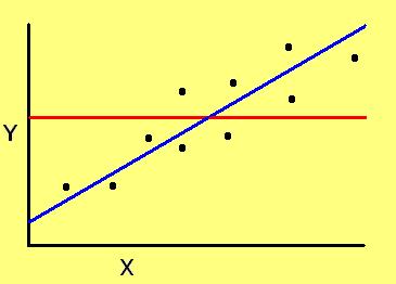
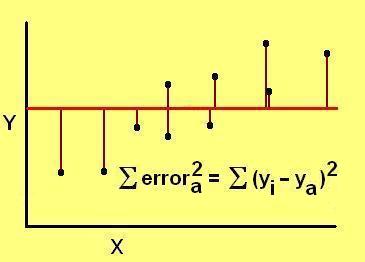
On the other hand, if there is a pattern, then we should be able to track it. The simplest pattern is a line, y = mx + b, where m = slope of the line, and b= y-intercept of the line when x = 0. We justify that the data follow a linear pattern by showing that using the line results in less error than using a simple arithmetic average. This is known as the goodness-of-fit of the line, and it is numerically expressed by the correlation coefficient (r2):
|
|
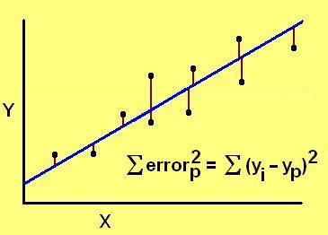
If the predicted line has less error than the average value, then its distance from the measured value will usually be smaller than the distance between the average value and the measured value. Summed across all the points, it will definitely yield a smaller number, the numerator will be smaller than the denominator, and the value of r2 will be close to 1.00. A perfect fit by a line will have r2 = 1.00, whereas a poor fit by a line will have a low value. If r2 = 0, then the predicted line is no better than a simple average of the data collected. With all linear predictions r2 < 1, always.
This is easy enough to do by hand. It is even easier today with computers that do it for us.