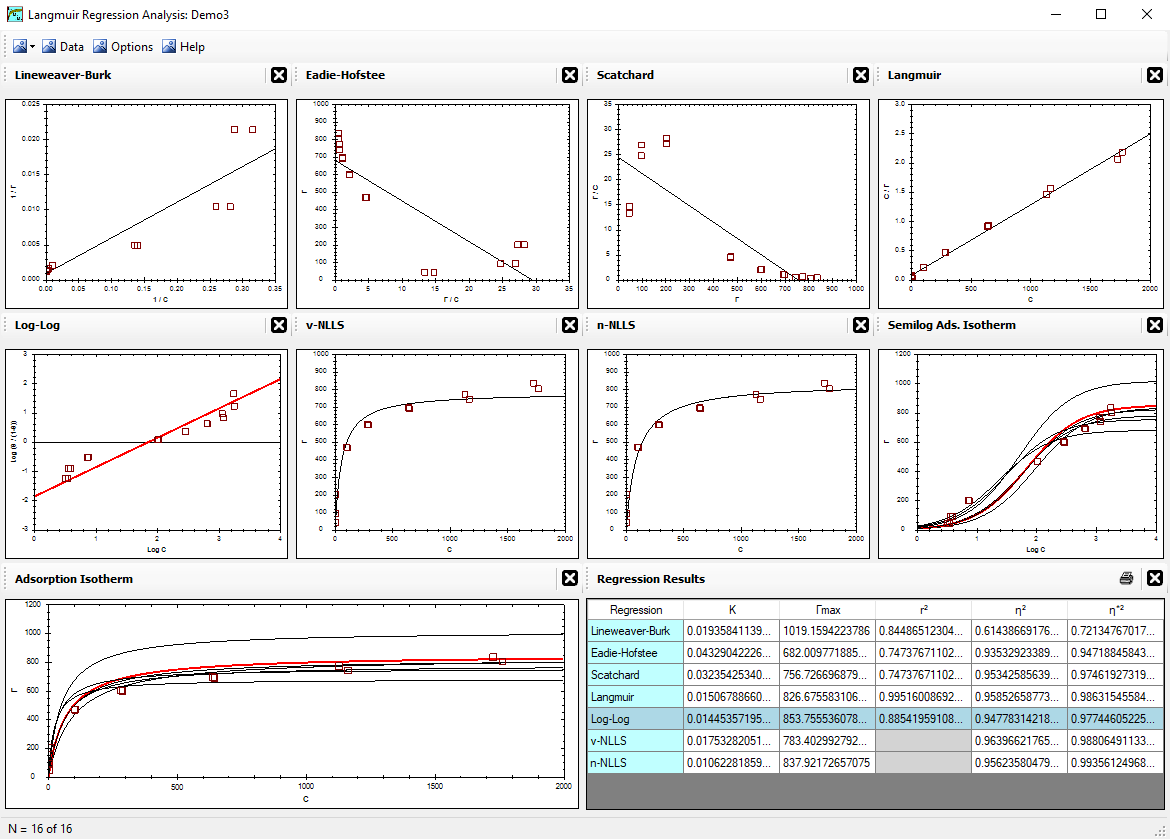
The Langmuir Optimization Program
| Alfisol, Item 003: | LMMpro, version 2.0 The Langmuir Optimization Program |
|

|
|
We could randomly guess the m and b values of the line, tabulate the error of each, and then identify which guess results in the least error. This can be done with a computer, but due to the lack of computers in the late 1700's, an alternate method was proposed that is much better. The method is called a least squares linear regression method because we solve the problem backwards (hence the term "regression"); that is, we first minimize the error and we then find out which line is it that gives us that low error value. The method does not really care what the minimum error value actually is. Instead, we note that the derivative of the error function reaches a minimum and its slope is equal to zero when the error value is also at a minimum.
| , and |
|
|
dε2
dm | = 0 = 2mΣxi2 + 2bΣxi - 2Σ(xiyi) |
|
dε2
db | = 0 = 2mΣxi + 2Σb - 2Σyi |
| m = |
Sxy - b Sx
Sxx |
We will use this optimization of slope in step 10 below, where it is used in combination with the intercept optimization. Do not use this equation to solve for m when the intercept's value b is fixed. Similarly, do not rearrange this equation to solve for b when the slope m is fixed. For these situations, use step 9 instead. Although by definition the sum of the square of the errors is minimized in step 5, optimizing the slope in step 5 does not necessarily result in a regression line whose sum of the errors is also zero because here a zero value for the sum of the errors depends on b.
b = (Sy - m Sx) / n .
Or, stated differently, Sy = mSx + nb.
If the slope's value m is fixed, then all parameters are known, and solve for b. If the intercept's value b is fixed, rearrange this equation, and solve for m. Although by definition the sum of the square of the errors is minimized in step 6, it is important to note that this time it also results in a regression line whose sum of the errors is zero for any value of b or m chosen. That is, the regression line resulting from step 6 will be arithmetically balanced as long as one of the two parameters (b or m) can be adjusted.
0 = m Sxx + Sx (Sy - m Sx)/n - Sxy
0 = m Sxx + SxSy/n - m SxSx/n - Sxy
0 = mn Sxx + SxSy - m SxSx - n Sxy
m (n Sxx - SxSx) = n Sxy - SxSy
| m = |
n Sxy - Sx Sy
n Sxx - Sx Sx |
Now plug this optimized value of m into step 9 to get the optimized value of b. This regression line will have a minimum value for the sum of the square of the errors, and a zero value for the sum of the errors.
This regression analysis is easy enough to do by hand. It is even easier today with computers that do it for us.
Note that this method was discovered by Carl Friedrich Gauss in 1795 (as noted by Gauss in his publication of the method in 1809). He was 17 years old at the time. The method was, however, first published by Adrien-Marie Legendre in 1805, and the most famous priority controversy in statistics followed Gauss's 1809 publication and comments about his developing it in 1795. It is a sad truth about priorities, but Gauss would have been recognized as the founder of many discoveries if only he had not been so slow in getting his ideas published (such as on complex analysis but Cauchy published it first, or on theory of elliptical functions but Abel and Jacobi published it first, and or on non-Euclidean geometry but Lobachevsky and Bolyai published it first). On the other hand, it is also known that Gauss was openly involved in the detailed development of the theory of least squares for many years. For more information on the history of linear regressions, review the translation of Gauss's memoirs by Stewart (1995) and the translator's excellent discussion and comments therein. See also Stigler (1981).
<Reference = CTT-6>