The Langmuir Optimization Program
| Alfisol, Item 003: | LMMpro, version 2.0 The Langmuir Optimization Program |
|
|
| Name of Linear Regression: | Langmuir Equation (1916):
Γ = Amount adsorbed Γmax = Maximum adsorption quantity K = Reaction equilibrium constant c = Aqueous Equilibrium concentration |
Michaelis-Menten Equation (1913):
v = Overall rate of reaction Vmax = Maximum reaction rate KM = Michaelis-Menten constant S = Substrate concentration |
Comments:
Note: the term "original graph" in the comments below refers to graph generated by either of the two parabolic equations expressed here, namely the Langmuir Equation or the Michaelis-Menten Equation, plus the (c, Γ) or the (S, v) original data. | ||||||||||||
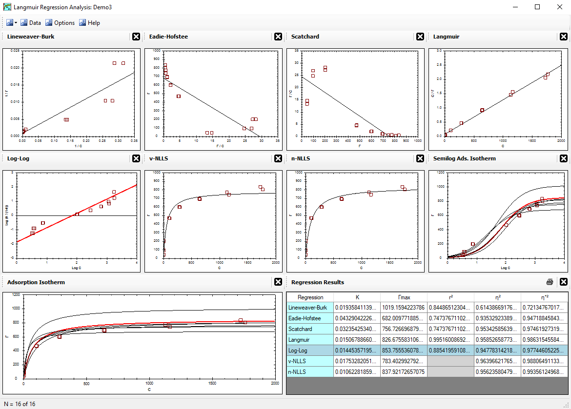
| Lineweaver-Burk (1934): |
plot (1/Γ) versus (1/c) slope = 1/(Γmax K) intercept = 1 / Γmax |
plot (1/v) versus (1/S) slope = KM / Vmax intercept = 1 / Vmax |
This regression method is extremely sensitive to data error.
It has a very strong bias for closely tracking the data in the lower left corner of the original graph. | ||||||||||||
| Eadie-Hofstee (1942, 1952): |
plot (Γ) versus (Γ/c) slope = -1 / K intercept = Γmax |
plot (v) versus (v/S) slope = -KM intercept = Vmax |
This regression method has some sensitivity to data error.
It has some bias for closely tracking the data in the lower left corner of the original graph.
Note that if you invert the x,y-axes, then this would
convert into the Scatchard regression. | ||||||||||||
| Scatchard (1949): |
plot (Γ/c) versus (Γ) slope = -K intercept = K Γmax |
plot (v/S) versus (v) slope = -1/KM intercept = Vmax / KM |
This regression method has some sensitive to data error.
It has some bias for closely tracking the data in the upper right corner of the original graph.
Note that if you invert the x,y-axes, then this would
convert into the Eadie-Hofstee regression. | ||||||||||||
| left: Langmuir (1918) right: Hanes-Woolf (1932, 1957): |
plot (c/Γ) versus (c) slope = 1 / Γmax intercept = 1/(K Γmax) |
plot (S/v) versus (S) slope = -1 / Vmax intercept = KM / Vmax |
This regression method has very little sensitivity to data error.
It has some bias for closely tracking the data in the middle portion of the graph plus the upper right corner of the original graph. This linear regression technique was first presented by Langmuir in 1918. Although he received the Nobel Prize in 1932, the method he used to optimize the parabolic equation was apparently totally missed by others. It was later presented by Hanes (1932) and referred to as the Hanes-Woolf regression by Haldane (1957), and this regression method often carries their names. This software (LMMpro) refers to this regression method as the "Langmuir Linear Regression Method" when used to solve the Langmuir adsorption isotherm. | ||||||||||||
| log-log: |
plot (log [θ/(1-θ)]) versus (log c) θ = Γ / Γmax slope = 1 intercept = log K |
plot (log [θ/(1-θ)]) versus (log S) θ = v/ Vmax slope = 1 intercept = -log KM |
This regression method has very little sensitivity to data error.
This is the only linear regression method that is too difficult to solve by hand. It must be solved via an iterative loop that finds the equation's best maximum value (and, hence, the best θ value). The best θ value is the one with the smallest linear regression error. Note that the slope is fixed and it is set equal to 1.0. |
Note that all linear and nonlinear regression methods are also sensitive to theory error. That is, a small deviation in the data from the Langmuir theory predictions or Michaelis-Menten theory preditions is not necessarily an expression of an error in the data collected. It may instead be due to a slightly incomplete mathematical expression of the true nature of the process involved.